Introduction
Consider an infinite small material volume in an arbitrary point of a structure. The infinite small material volume deforms exhibiting a certain strain pattern if it is submitted to a stress pattern with limited value. Stress patterns in an arbitrary material volume of a structure originate from internal forces in the material induced by external structural loads. If the value of the stress pattern is lower than a given limit, the material volume returns to its original shape when the external loads are removed. The deformation of the material volume (thus its stress-strain relationship) in this case can be described by its elastic material properties. If the value of the stress in a material point exceeds the limited value, a permanent deformation of the material volume can occur and the deformation can no longer be described only with the elastic material properties. The Engineering constants describe the elastic material behavior in a material volume. The Engineering constants are the Young’s moduli, Poisson’s ratios and shear moduli. If the values of the Young’s moduli and shear moduli are big, the material is called “stiff”, otherwise it is called “flexible”.
The “resonalyser procedure” is a mixed numerical-experimental method for identifying the Engineering Constants of thin 2D material sheets having elastic isotropic or orthotropic elastic properties. Material sheets include rectangular test beams and rectangular test plates with constant thickness over the entire sheet. The material elastic properties are assumed to be uniform in all points of the sheets. For orthotropic materials, the material symmetry axes are assumed to be parallel (or perpendicular) with the sheet boundaries.
The basic principle of the “resonalyser procedure” is to measure the vibration behavior of the test sheets and to compare these measurements with computed vibration behavior. Accurate finite element models of the test sheets are used to compute the vibration behavior. The engineering constants in the finite element models are tuned in such a way that the computed vibration behavior matches the measured vibration behavior as close as possible. The vibration behavior can be represented by a limited series of natural frequencies of the test sheets.
Isotropic and Orthotropic elastic material properties
For a beam (a one dimensional sheet), the dominating Engineering constants are the Young’s modulus E in the longitudinal direction and Poisson’s ratio ν.
Standard testing for measuring the Engineering Constants of beams is often performed by a tensile test on a test beam equipped with strain gages (or a similar deformation sensor).
It is assumed that all material points of the beam material during a tensile test have a uniform stress σ and a uniform strain ε. The relationship between the stress σ and the strain ε is given by the formulas below. F is the tensile force, A is the cross section area, E is the Young’s modulus and ΔL is the extra deformation of the original sensor gauge length L0 .
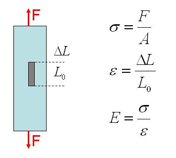
Poisson’s ratio can be measured if also the (negative) transverse strain is measured with the sensor. Poisson’s ratio is defined as the negative ratio of the transverse and longitudinal strain.
The elastic properties of a material volume are called isotropic if the Engineering constants are the same in all possible directions of the considered material volume. Examples of isotropic material are commonly known materials like glass, cement, metals, plastics, and short fiber reinforced plastics with random distribution and so on… For a two dimensional sheet, the relations between in-plane stresses and strains are given by the flexibility matrix. In the case of 2D plane stress this relation can be written for isotropic material as:
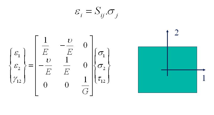
ε1 and ε2 are the normal strains and γ12 is the in-plane shear angle in the sheet material axe system (1, 2). σ1 and σ2 are the normal stresses. E is the Young’s modulus, G is the in-plane shear modulus and ν is the Poisson’s ratio. The following relation for the shear modulus G is valid for isotropic material behavior:
G =E/2(1 + ν)
So there are only two independent Engineering constants to be determined in order to characterize the elastic properties of an isotropic material.
A material is called orthotropic when the elastic properties are symmetric with respect to a rectangular Cartesian system of axes. In the Resonalyser procedure the material symmetry axes are supposed to be parallel (or perpendicular) with the sheet boundaries. In case of 2D plane stress, the stress-strain relations for orthotropic material become:
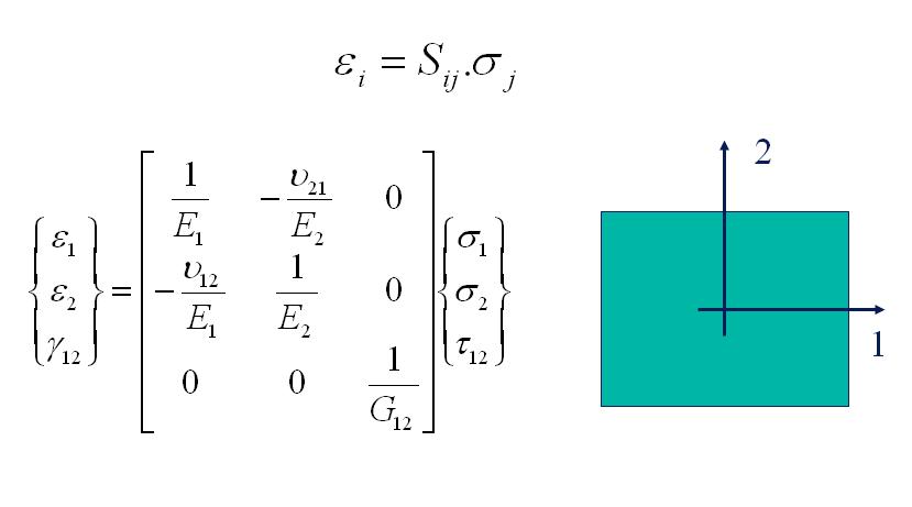
ε1 and ε2 are the normal strains and γ12 is the in-plane shear angle in the orthotropic material axe system (1, 2). σ1 and σ2 are the normal stresses. E1 and E2 are the Young’s moduli in the 1- and 2-direction and G12 is the in-plane shear modulus. ν12 is the major Poisson’s ratio and ν21 is the minor Poisson’s ratio. The flexibility matrix is symmetric. The minor Poisson’s ratio can hence be found if E1, E2 and ν12 are known.
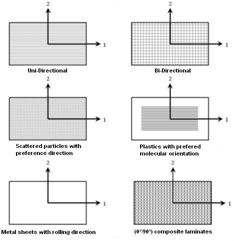
The figure above shows some examples of common orthotropic materials: layered uni-directionally reinforced composites with fiber directions parallel to the plate edges, layered bi-directionally reinforced composites, short fiber reinforced composites with preference directions (like wooden particle boards), plastics with extrusion preference orientation, rolled metal sheets, and much more…
Standard methods for the identification of the two Young’s moduli E1 and E2 require two tensile tests, one on a beam cut along the 1-direction and one on a beam cut along the 2-direction. Major and minor Poisson’s ratio’s can be identified if also the transverse strains are measured during the tensile tests. The identification of the in-plane shear modulus requires an additional in plane shearing test.
The Impulse Excitation Technique (IET) is an alternative method that can identify the Engineering constants of isotropic materials. A test beam is impacted with an impulse (for example using a hammer) and the response of the beam is measured with a sensor (a microphone, a laser vibrometer or an accelerometer). The natural frequency of the beam is derived using a Fourier analysis software package. The engineering constants can be computed using analytical formula’s relating the measured natural frequency with an engineering constant.
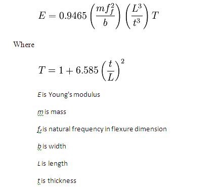
In case the natural frequency f is measured for a bending (“flexural”) modal shape on a thin beam with a rectangular cross section (b x t), a Length L and a Mass M, the formula for Young’s Modulus E below is used.
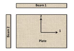
 The “resonalyser procedure” is an extension of the IET allowing a fast and accurate simultaneous identification of the 4 Engineering constants E1, E2, G12 and v12 for orthotropic materials and the 2 Engineering constants E and G in the case of isotropic materials. For the identification of the four orthotropic material constants, the first three natural frequencies of a rectangular test plate with constant thickness and the first natural frequency of two test beams with rectangular cross section must be measured. One test beam is cut along the longitudinal direction, the other one cut along the transversal direction (see Figure below).
The Young’s modulus of the test beams can be found using the IET formula for test beams with a rectangular cross section.
The ratio Width/Length of the test plate must be cut according to the following formula:
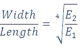
This ratio yields a so-called “Poisson plate”. The first 3 natural frequencies of a Poisson plate are sensitive for variations of all the orthotropic Engineering constants.
The Resonalyser procedure for material identification consists of the following steps:
- Measurement of the Length and natural frequencies of the test beams
- Defining the aspect ratio L1/L2 for a Poisson plate and producing such a test plate
- Measurement of the 3 first natural frequencies of the Poisson plate
- Identification of the 4 orthotropic Engineering constants using a finite element models of the two Beams and the Poisson plate
Some background about natural frequencies is given in the next paragraph. The practical measurement of the natural frequency is explained in the help function of the measurement form.
Vibration of beams and rectangular plates
The vibration of beams and rectangular plates can be characterized by their modal shapes and the associated natural frequencies. The figure below shows the fundamental bending modal shape of a beam with uniform thickness. A modal shape is a standing wave vibrating at a natural frequency. In one vibration period, the beam undergoes a deformation starting from a non deformed shape to a maximum deformation in one transverse direction, next a maximal deformation in the opposite transverse direction and finally the beam returns to the non deformed shape. The natural frequency indicates how many such vibration periods the beam performs in one second. The number of cycles is expressed in Hertz. One Hertz equals one period in one second. The value of the natural frequency which is associated to the modal shape vibration pattern is high for stiff beams with a relative small mass and low for flexible beams with a relative high mass.
Basic Modal bending shape
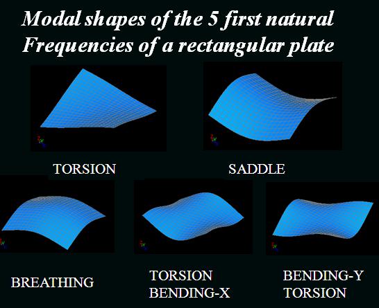
The figure below shows the modal shapes associated with the first 5 natural frequencies of a rectangular plate.
Natural frequencies and their modal shapes can be measured experimentally and can be computed as well using numerical computer models. A very powerful numerical modal is the finite element model. Next paragraph gives some background information about finite element models and how to compute vibration behavior using a finite element computer model.
Finite Element models of beams and plates
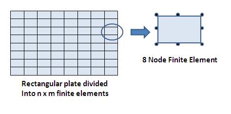
The finite element method divides a structure into a big number of sub domains called “Finite Elements”. In the example below, a rectangular plate is divided into n x m finite elements. This is called the finite element model of the plate. The geometry of each element can be defined by nodes. In the example below, a finite element is defined by 8 nodes.
Each node of an element can be associated with an interpolation function, usually called “shape functions”. A shape function has the property to have the value 1 in the node where it is defined and zero in all other nodes of the element. The figure below shows the shape functions of an 8 node element.
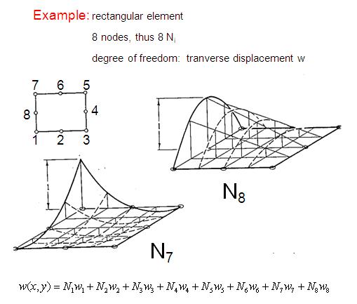
The degree of freedom in an arbitrary point of the sub domain of a finite element can be expressed as a summation of the value of the degree of freedom in the nodes multiplied with their shape function. The relation between bending and torsion moments acting on a plate and the plate curvatures they are causing is established by the plate rigidity matrix.
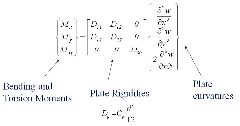
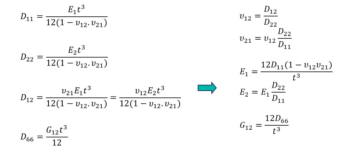
The plate rigidities can be found by the thickness t of the plate and the engineering constants. Vice versa, the Engineering constants can be found if the plate rigidities are known. In the formulas below, it is assumed that the material properties are uniform in the thickness direction.
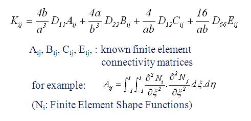
The finite element stiffness matrix of a finite element [K]e can be composed by connectivity matrices and the plate rigidities.
Using the geometry, mass information and the shape functions, the finite element method can evaluate also a Mass matrix [M]e for each element. All these element matrices can next be assembled to form the total structure finite element matrices [K] and [M] of a plate (beam). The natural frequencies ƒi of the plate (beam) and the associated modal shapes φ can be computed from these matrices by the solution of an eigenvalue problem (see figure below).
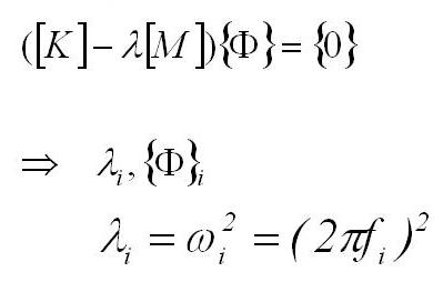
The solution of the eigenvalue problem yields N eigenvalues λ and the associated modal shapes φ (an eigenvalue couple). N is the number of degrees of freedom of the finite element model. The natural frequencies can be computed from the eigenvalues. Only the first 3 (or sometimes 5) first eigenvalue couples are used in the resonalyser procedure. The Engineering constants in the stiffness matrix are tuned in such a way that the computed natural frequencies match the measured natural frequencies.
Tuning the Engineering constants in the finite element model is performed by a mixed numerical experimental method and is described in the next paragraph.
Mixed numerical-experimental procedures (inverse methods)
The resonalyser procedure is a so called “Mixed Numerical-experimental procedure” or also called an “inverse method”. The principle is to tune the Elastic Engineering constants in a finite element of the Poisson test plate in such a way that the computed values of the natural frequencies (by the solution of an eigenvalue problem) match the measured natural frequencies as close as possible. An inverse method like the resonalyser procedure hence need measured values of the test plate, a finite element model of the same test plate and an updating algorithm. The updating algorithm aims to reduce the difference between a set of computed natural frequencies and measured natural frequencies. The difference is store in the so-called “output residual”.
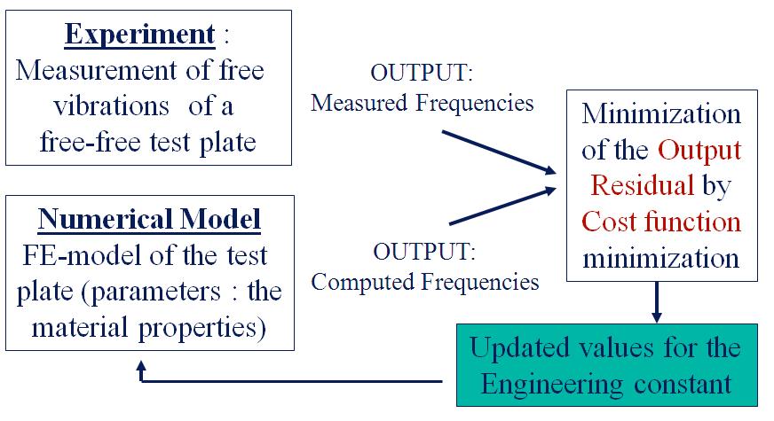
A scalar value (called “the cost function”) is minimized by the algorithm in an iterative way. The procedure starts with initial values for the Engineering constants. These values are iteratively updated till the cost function (and hence the output residual) are minimal. The values of the Engineering constants that minimize the cost function are the solution values of the Resonalyser procedure.
Identification of the damping behavior of the material
In the case of visco-elastic material behavior the Resonalyser procedure can also identify the complex engineering constants. The complex engineering constants have a real and an imaginary part. The real part describes the elastic behavior and the imaginary part (the so-called “tangents delta”) describes the damping behavior.
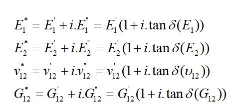
The real part can be identified using the resonance frequencies in the Resonalyser procedure (see previous paragraph). The imaginary part can be identified by measuring the modal damping ratios (ξBeam1 and ξBeam2) associated with fundamental bending modal shapes of the two beams and the modal damping ratios (ξTorsion ξSaddle and ξBreathing) associated with the 3 modal shapes of the Poisson plate.
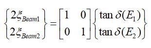
The bending modal shape of the beams is directly proportional with the tangents delta of the Young’s moduli E1 and E2.
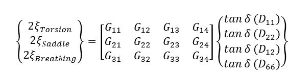
For the plate, each of the modal shapes receives a contribution of the 4 plate rigidities. The relation is given by the G matrix, which contains components related to the modal strain energy of the modal shapes. The G matrix can be computed by the finite element program in the Resonalyser software using the identified real part of the engineering constants.
By using the relation between the plate rigidities and the engineering constants, the tangents deltas of the plate rigidities and all the engineering constants can be solved.
This means that all the complete complex engineering constants can be found in two steps: a first step is the identification of the real part using measured frequencies and the second step is the identification of the imaginary part using the measured modal damping ratios.
More theoretical details about the resonalyser method can be found in the list of references.
References: Knowledge Articles